New R package yfR

Facilitating download of stock data from Yahoo Finance

2022-03-31 9 min read R, yfR, BatchGetSymbols

Package BatchGetSymbols facilitates importation of Yahoo Finance data directly into R and is one of my most popular R packages, with over 100k installations since conception (around 2500 downloads per month). However, I developed BatchGetSymbols back in 2016, with many bad structural choices from my part.

For years I wanted to improved the code but always restrained myself because I did not want to mess up the execution of other people’s code that was based on BatchGetSymbols. In order to implement all the breaking changes and move forward with the package, I decided to develop a new (and fresh) package called yfR.

Today I’m releasing the first version of yfR (not yeat in CRAN). This in a major upgrade on BatchGetSymbols, with many backwards-incompatible changes.

Motivation

yfR is the second and backwards-incompatible version of BatchGetSymbols. In a nutshell, it provides access to daily stock prices from Yahoo Finance, a vast repository with financial data around the globe. Yahoo Finance cover a large number of markets and assets, being used extensively for importing price datasets used in academic research and teaching.

Package yfR is based on quantmod and used its main function for fetching data from Yahoo Finance. The main innovation in yfR is in the organization of the imported financial data and using local caching system and parallel computing for speeding up large scale download of datasets from Yahoo Finance.

See full documentation here.

Features

Fetchs daily/weekly/monthly/annual stock prices/returns from yahoo finance and outputs a dataframe (tibble) in the long format (stacked data);
A new feature called “collections” facilitates download of multiple tickers from a particular market/index. You can, for example, download data for all stocks in the SP500 index with a simple call to yf_collection_get();
A session-persistent smart cache system is available by default. This means that the data is saved locally and only missing portions are downloaded, if needed.
All dates are compared to a benchmark ticker such as SP500 and, whenever an individual asset does not have a sufficient number of dates, the software drops it from the output. This means you can choose to ignore tickers with high number of missing dates.
A customized function called yf_convert_to_wide() can transform the long dataframe into a wide format (tickers as columns), much used in portfolio optimization. The output is a list where each element is a different target variable (prices, returns, volumes).
Parallel computing with package furrr is available, speeding up the data importation process.

Differences from BatchGetSymbols

Package BatchgetSymbols was developed back in 2016, with many bad structural choices from my part. Since then, I learned more about R and its ecosystem, resulting in better and more maintainable code. However, it is impossible to keep compatibility with the changes I wanted to make, which is why I decided to develop a new (and fresh) package.

Here are the main differences between yfR (new) and BatchGetSymbols (old):

All input arguments are now formatted as “snake_case” and not “dot.case”. For example, the argument for the first date of data importation in yfR::yf_get() is first_date, and not first.date as used in BatchGetSymbols::BatchGetSymbols.
All function have been renamed for a common API notation. For example, BatchGetSymbols::BatchGetSymbols is now yfR::yf_get(). Likewise, the function for fetching collections is yfR::yf_collection_get().
The output of yfR::yf_get() is always a tibble with the price data (and not a list as in BatchGetSymbols::BatchGetSymbols). If one wants the tibble with a summary of the importing process, it is available as an attribute of the output (see function base::attributes)
A new feature called “collection”, which allows for easy download of a collection of tickers. For example, you can download price data for all components of the SP500 by simply calling yfR::yf_collection_get("SP500").
New and prettier status messages using package cli

You can find more details at its github repo:

https://github.com/msperlin/yfR

Installation

# CRAN (not yet available)
#install.packages('yfR')

# Github (dev version)
devtools::install_github('msperlin/yfR')

Examples

Fetching a single stock price

library(yfR)

# set options for algorithm
my_ticker <- 'FB'
first_date <- Sys.Date() - 30
last_date <- Sys.Date()

# fetch data
df_yf <- yf_get(tickers = my_ticker, 
                first_date = first_date,
                last_date = last_date)

##

## ── Running yfR for 1 stocks | 2022-03-01 --> 2022-03-31 (30 days) ──

##

## ℹ Downloading data for benchmark ticker ^GSPC

## ℹ (1/1) Fetching data for ',
## 'FB

## !    - not cached

## ✓    - cache saved successfully

## ✓    - got 22 valid rows (2022-03-01 --> 2022-03-30)

## ✓    - got 100% of valid prices -- Well done msperlin!

## ℹ Binding price data

# output is a tibble with data
head(df_yf)

## # A tibble: 6 × 10
##   ticker ref_date   price_open price_high price_low price_close   volume
##   <chr>  <date>          <dbl>      <dbl>     <dbl>       <dbl>    <dbl>
## 1 FB     2022-03-01       210.       212.      202.        203. 27094900
## 2 FB     2022-03-02       205.       209.      202.        208. 29452100
## 3 FB     2022-03-03       209.       209.      201.        203. 27263500
## 4 FB     2022-03-04       202.       206.      199.        200. 32130900
## 5 FB     2022-03-07       201.       201.      187.        187. 38560600
## 6 FB     2022-03-08       188.       197.      186.        190. 37508100
## # … with 3 more variables: price_adjusted <dbl>, ret_adjusted_prices <dbl>,
## #   ret_closing_prices <dbl>

Fetching many stock prices

library(yfR)
library(ggplot2)

my_ticker <- c('FB', 'GM', 'MMM')
first_date <- Sys.Date() - 100
last_date <- Sys.Date()

df_yf_multiple <- yf_get(tickers = my_ticker, 
                         first_date = first_date,
                         last_date = last_date)

##

## ── Running yfR for 3 stocks | 2021-12-21 --> 2022-03-31 (100 days) ──

##

## ℹ Downloading data for benchmark ticker ^GSPC

## ℹ (1/3) Fetching data for ',
## 'FB

## ✓    - found cache file (2022-03-01 --> 2022-03-30)

## !    - need new data (cache doesnt match query)

## ✓    - got 69 valid rows (2021-12-21 --> 2022-03-30)

## ✓    - got 100% of valid prices -- All OK!

## ℹ (2/3) Fetching data for ',
## 'GM

## !    - not cached

## ✓    - cache saved successfully

## ✓    - got 69 valid rows (2021-12-21 --> 2022-03-30)

## ✓    - got 100% of valid prices -- Well done msperlin!

## ℹ (3/3) Fetching data for ',
## 'MMM

## !    - not cached

## ✓    - cache saved successfully

## ✓    - got 69 valid rows (2021-12-21 --> 2022-03-30)

## ✓    - got 100% of valid prices -- Youre doing good!

## ℹ Binding price data

p <- ggplot(df_yf_multiple, 
            aes(x = ref_date, y = price_adjusted,
                color = ticker)) + 
  geom_line()

print(p)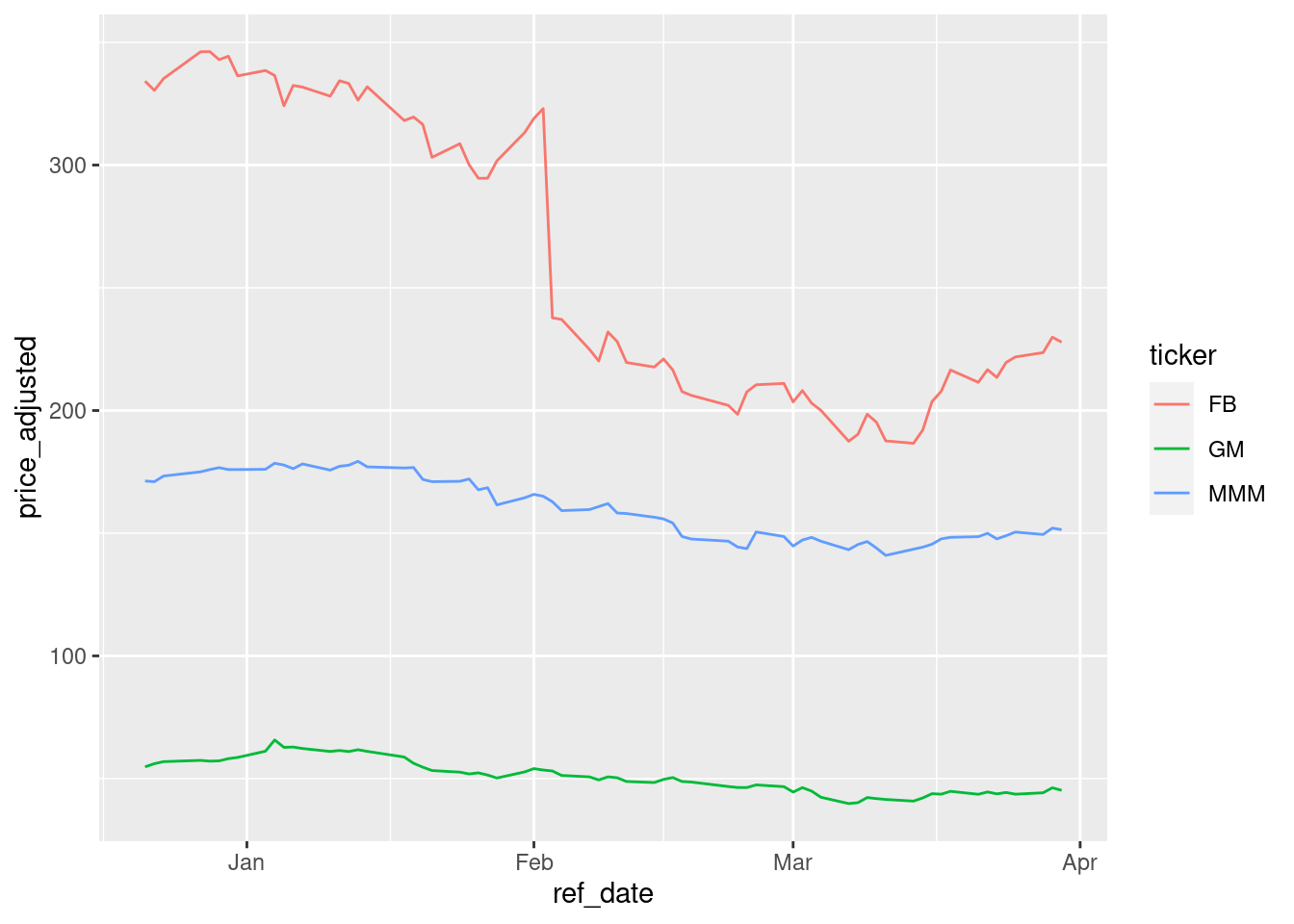

Fetching collections of prices

Collections are just a bundle of tickers pre-organized in the package. For example, collection SP500 represents the current composition of the SP500 index.

library(yfR)

df_yf <- yf_collection_get("SP500", 
                           first_date = Sys.Date() - 30,
                           last_date = Sys.Date())

head(df_yf)

Fetching daily/weekly/monthly/yearly price data

library(yfR)
library(ggplot2)
library(dplyr)

## 
## Attaching package: 'dplyr'

## The following objects are masked from 'package:stats':
## 
##     filter, lag

## The following objects are masked from 'package:base':
## 
##     intersect, setdiff, setequal, union

my_ticker <- 'GE'
first_date <- '2010-01-01'
last_date <- Sys.Date()

df_dailly <- yf_get(tickers = my_ticker, 
                    first_date, last_date, 
                    freq_data = 'daily') |>
  mutate(freq = 'daily')

##

## ── Running yfR for 1 stocks | 2010-01-01 --> 2022-03-31 (4472 days) ──

##

## ℹ Downloading data for benchmark ticker ^GSPC

## ℹ (1/1) Fetching data for ',
## 'GE

## !    - not cached

## ✓    - cache saved successfully

## ✓    - got 3082 valid rows (2010-01-04 --> 2022-03-30)

## ✓    - got 100% of valid prices -- Time for some tea?

## ℹ Binding price data

df_weekly <- yf_get(tickers = my_ticker, 
                    first_date, last_date, 
                    freq_data = 'weekly') |>
  mutate(freq = 'weekly')

##

## ── Running yfR for 1 stocks | 2010-01-01 --> 2022-03-31 (4472 days) ──

##

## ℹ Downloading data for benchmark ticker ^GSPC

## ℹ (1/1) Fetching data for ',
## 'GE

## ✓    - found cache file (2010-01-04 --> 2022-03-30)

## ✓    - got 3082 valid rows (2010-01-04 --> 2022-03-30)

## ✓    - got 100% of valid prices -- You got it msperlin!

## ℹ Binding price data

df_monthly <- yf_get(tickers = my_ticker, 
                     first_date, last_date, 
                     freq_data = 'monthly') |>
  mutate(freq = 'monthly')

##

## ── Running yfR for 1 stocks | 2010-01-01 --> 2022-03-31 (4472 days) ──

##

## ℹ Downloading data for benchmark ticker ^GSPC

## ℹ (1/1) Fetching data for ',
## 'GE

## ✓    - found cache file (2010-01-04 --> 2022-03-30)

## ✓    - got 3082 valid rows (2010-01-04 --> 2022-03-30)

## ✓    - got 100% of valid prices -- Good stuff!

## ℹ Binding price data

df_yearly <- yf_get(tickers = my_ticker, 
                    first_date, last_date, 
                    freq_data = 'yearly') |>
  mutate(freq = 'yearly')

##

## ── Running yfR for 1 stocks | 2010-01-01 --> 2022-03-31 (4472 days) ──

##

## ℹ Downloading data for benchmark ticker ^GSPC

## ℹ (1/1) Fetching data for ',
## 'GE

## ✓    - found cache file (2010-01-04 --> 2022-03-30)

## ✓    - got 3082 valid rows (2010-01-04 --> 2022-03-30)

## ✓    - got 100% of valid prices -- Good job msperlin!

## ℹ Binding price data

df_allfreq <- bind_rows(
  list(df_dailly, df_weekly, df_monthly, df_yearly)
) |>
  mutate(freq = factor(freq, 
                       levels = c('daily', 
                                  'weekly',
                                  'monthly',
                                  'yearly'))) # make sure the order in plot is right

p <- ggplot(df_allfreq, aes(x=ref_date, y = price_adjusted)) + 
  geom_point() + geom_line() + facet_grid(freq ~ ticker) + 
  theme_minimal() + 
  labs(x = '', y = 'Adjusted Prices')

print(p)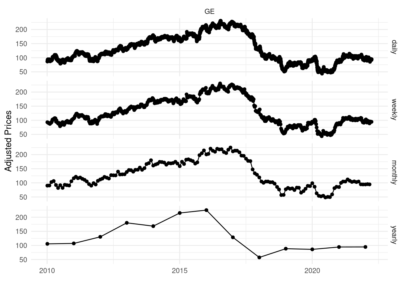

Changing format to wide

library(yfR)
library(ggplot2)

my_ticker <- c('FB', 'GM', 'MMM')
first_date <- Sys.Date() - 100
last_date <- Sys.Date()

df_yf_multiple <- yf_get(tickers = my_ticker, 
                         first_date = first_date,
                         last_date = last_date)

##

## ── Running yfR for 3 stocks | 2021-12-21 --> 2022-03-31 (100 days) ──

##

## ℹ Downloading data for benchmark ticker ^GSPC

## ℹ (1/3) Fetching data for ',
## 'FB

## ✓    - found cache file (2021-12-21 --> 2022-03-30)

## ✓    - got 69 valid rows (2021-12-21 --> 2022-03-30)

## ✓    - got 100% of valid prices -- Good job msperlin!

## ℹ (2/3) Fetching data for ',
## 'GM

## ✓    - found cache file (2021-12-21 --> 2022-03-30)

## ✓    - got 69 valid rows (2021-12-21 --> 2022-03-30)

## ✓    - got 100% of valid prices -- All OK!

## ℹ (3/3) Fetching data for ',
## 'MMM

## ✓    - found cache file (2021-12-21 --> 2022-03-30)

## ✓    - got 69 valid rows (2021-12-21 --> 2022-03-30)

## ✓    - got 100% of valid prices -- Well done msperlin!

## ℹ Binding price data

l_wide <- yf_convert_to_wide(df_yf_multiple)

prices_wide <- l_wide$price_adjusted

head(prices_wide)

## # A tibble: 6 × 4
##   ref_date      FB    GM   MMM
##   <date>     <dbl> <dbl> <dbl>
## 1 2021-12-21  334.  54.8  171.
## 2 2021-12-22  330.  56.1  171.
## 3 2021-12-23  335.  56.9  173.
## 4 2021-12-27  346.  57.4  175.
## 5 2021-12-28  346.  57.1  176.
## 6 2021-12-29  343.  57.2  177.

R yfR BatchGetSymbols

Marcelo S. Perlin

Associate Professor

My research interests include data analysis, finance and cientometrics.