5 Importing Data from the Internet
One of the great advantages of using R in Finance and Economics is the large amount of data that can be imported using the internet, substituting the tedious, unreliable and soul-crushing work of manual data collection. It also becomes easier to share reproducible code, as anyone can feasibly download the same tables with a single line of code.
In this chapter, we will study the most important and reliable packages for data importation in the fields of Finance and Economics. It is a small, but comprehensive list of packages that cover a large range of research topics. The list includes:
- {GetQuandlData} (M. S. Perlin 2023b)
- Imports economical and financial data from the Quandl platform.
- {yfR} (M. Perlin 2023)
- Imports adjusted and unadjusted stock price data from Yahoo Finance.
- {simfinapi} (Gomolka 2023)
- Imports financial statements and adjusted stock prices from the SimFin project40.
- {tidyquant} (Dancho and Vaughan 2023)
- Imports several financial information about stock prices and fundamental data.
5.1 Package {GetQuandlData}
Quandl is an established and comprehensive platform that provides access to a series of free and paid data. Several central banks and research institutions provide free economic and financial information on this platform. I strongly recommend browsing the available tables from the Quandl website41. It is likely that you’ll find datasets that you’re familiar with.
In R, package {Quandl} (Raymond McTaggart, Gergely Daroczi, and Clement Leung 2021) is the official extension offered by the company and available in CRAN. However, the package has some issues (see blog post here42), which are fixed with the alternative package {GetQuandlData} (M. S. Perlin 2023b).
The first and mandatory step in using {GetQuandlData} (M. S. Perlin 2023b) is to register a user at the Quandl website43. Soon after, go to account settings and click API KEY. This page should show a code, such as Asv8Ac7zuZzJSCGxynfG. Copy it to the clipboard (control + c) and, in R, define a character object containing the copied content as follows:
# set FAKE api key to quandl
my_api_key <- 'Asv8Ac7zuZzJSCGxynfG'
The API key is unique to each user, and the one presented here will not work on your computer. You’ll need to get your own API key to run the examples of the book. After finding and setting your key, go to Quandl’s website and use the search box to look for the symbol of the time series of interest. As an example, we will use data for gold prices in the London Market, with a Quandl code equivalent to 'LBMA/GOLD'. Do notice that the structure of a Quandl code is always the same, with the name of the main database at first, and the name of table second, separated by a forward slash (/).
Now, with the API key and the Quandl symbol, we use function GetQuandlData::get_Quandl_series() to download the data from 1980-01-01 to 2023-01-01:
# set symbol and dates
my_symbol <- c('GOLD' = 'LBMA/GOLD')
first_date <- '1980-01-01'
last_date <- '2023-01-01'

# get data!
df_quandl <- GetQuandlData::get_Quandl_series(
  id_in = my_symbol,
  api_key = my_api_key,
  first_date = first_date,
  last_date = last_date,
  do_cache = FALSE)

# check it
dplyr::glimpse(df_quandl)
R> Rows: 10,866
R> Columns: 9
R> $ `USD (AM)` <chr> "559", "632", "596", "634", "615.75", …
R> $ `USD (PM)` <chr> "559.5", "634", "588", "633.5", "610",…
R> $ `GBP (AM)` <chr> "251.123", "281.577", "266.285", "281.…
R> $ `GBP (PM)` <chr> "250.841", "282.468", "262.77", "280.0…
R> $ `EURO (AM)` <chr> NA, NA, NA, NA, NA, NA, NA, NA, NA, NA…
R> $ `EURO (PM)` <chr> NA, NA, NA, NA, NA, NA, NA, NA, NA, NA…
R> $ series_name <chr> "GOLD", "GOLD", "GOLD", "GOLD", "GOLD"…
R> $ ref_date <date> 1980-01-02, 1980-01-03, 1980-01-04, 1…
R> $ id_quandl <chr> "LBMA/GOLD", "LBMA/GOLD", "LBMA/GOLD",…Notice how we set the name of the time series in line id_in = c('GOLD' = 'LBMA/GOLD'). The name of the element becomes the value of column series_name in df_quandl. If we had more time series, they would be stacked in the same table, but with different series_name value.
There are other Quandl API options available with inputs order, collapse and transform. If using Quandl is important to your work, I strongly recommend reading the available parameters for querying data44. Several choices for data transformations can be passed to function GetQuandlData::get_Quandl_series() .
As an inspection check, let’s plot the prices of Gold in USD over time.
Overall, gold prices were fairly stable between 1980 and 2000, reaching a spike after 2010. One possible explanation is the higher demand for safer assets, such as gold, after the 2009 financial crisis.
5.2 Package {yfR}
Package {yfR} (M. Perlin 2023) is all about downloading stock price data from Yahoo Finance. Unlike other packages, {yfR} (M. Perlin 2023) focuses on large batch downloads of structured and clean/tidy data. Its main features are:
Fetches daily/weekly/monthly/annual stock prices/returns from yahoo finance and outputs a dataframe (tibble) in the long format (stacked data);
A feature called collections facilitates download of multiple tickers from a particular market/index. You can, for example, download data for all stocks in the SP500 index with a simple call to
yf_collection_get("SP500");A session-persistent smart cache system is available by default. This means that the data is saved locally and only missing portions are downloaded, if needed.
All dates are compared to a benchmark ticker such as SP500 and, whenever an individual asset does not have a sufficient number of dates, the software drops it from the output. This means you can choose to ignore tickers with a high proportion of missing dates.
A customized function called yfR::yf_convert_to_wide() can transform a long
dataframeinto a wide format (tickers as columns), much used in portfolio optimization. The output is a list where each element is a different target variable (prices, returns, volumes).Parallel computing with package
furrris available, speeding up the data importation process.
As an example of usage, let’s download the prices of four stocks in the previous five years using function yfR::yf_get() . We choose these companies: Microsoft (MSFT), Google (GOOGL), JP Morgan (JPM) and General Electric (GE).
In the call to function yfR::yf_get() , we set arguments thresh_bad_data = 0.95 and bench_ticker = '^GSPC'. These choices make sure that all returned data have at least 95% of valid prices when compared to data from the SP500 index (ticker '^GSPC').
# set tickers
tickers <- c('MSFT','GOOGL','JPM','GE')

# set dates
first_date <- Sys.Date()-5*365 # past five years
last_date <- Sys.Date()   # today
thresh_bad_data <- 0.95   # sets percent threshold for bad data
bench_ticker <- '^GSPC'   # set benchmark as SP500

df_yf <- yfR::yf_get(tickers = tickers,
                     first_date = first_date,
                     last_date = last_date,
                     bench_ticker = bench_ticker,
                     thresh_bad_data = thresh_bad_data)
The output of yfR::yf_get() is an object of type dataframe, a table with prices and returns:
# print df.tickers
dplyr::glimpse(df_yf)
R> Rows: 5,028
R> Columns: 11
R> $ ticker <chr> "GE", "GE", "GE", "GE", "GE…
R> $ ref_date <date> 2018-12-14, 2018-12-17, 20…
R> $ price_open <dbl> 42.51486, 42.57491, 43.1153…
R> $ price_high <dbl> 43.53570, 43.41560, 45.8175…
R> $ price_low <dbl> 42.03447, 42.09452, 42.9952…
R> $ price_close <dbl> 42.63496, 42.93521, 43.7158…
R> $ volume <dbl> 21449181, 21604120, 2444219…
R> $ price_adjusted <dbl> 41.77919, 42.07340, 42.8383…
R> $ ret_adjusted_prices <dbl> NA, 0.007042079, 0.01818195…
R> $ ret_closing_prices <dbl> NA, 0.007042277, 0.01818180…
R> $ cumret_adjusted_prices <dbl> 1.0000000, 1.0070421, 1.025…As expected, we find information about stock prices, daily returns and traded volumes. Notice it also includes column ticker, which contains the symbols of the stocks. In the tidy format, each stock has a chunk of data that is pilled in top of each other. Later, in chapter 8, we will use this column to split the data and build summary tables. To inspect the data, create a figure with the prices:
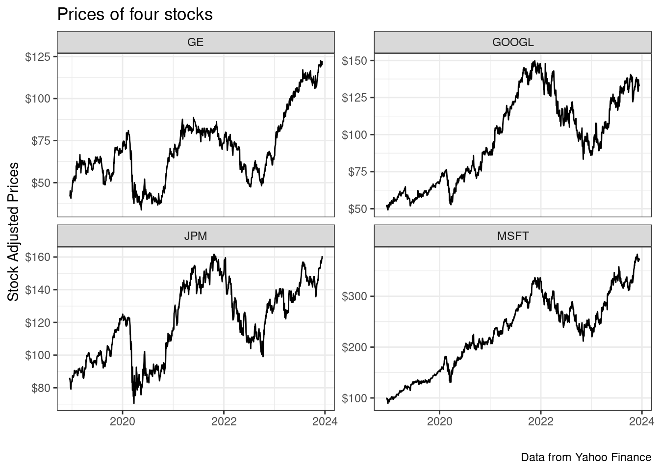
We see that General Eletric (GE) stock was not kind to its investors. Someone that bought the stock at its peak in mid-2016 has found its current value at less than half. Now, when it comes to the GOOGL, JPM and MSFT, we see an overall upward increase in stock prices, and a recent drop. These are profitable and competitive companies in their sectors and not surprisingly, the stock prices surged over the long period of time.
Now, let’s look at an example of a large download of stock price data. Here, we will download the current composition of the SP500 index using function yfR::yf_collection_get() .
# set dates
first_date <- '2020-01-01'
last_date <- '2023-01-01'

df_dow <- yfR::yf_collection_get(
  "DOW",
  first_date,
  last_date
)
And now we check the resulting data:
dplyr::glimpse(df_dow)R> Rows: 22,680
R> Columns: 11
R> $ ticker <chr> "AAPL", "AAPL", "AAPL", "AA…
R> $ ref_date <date> 2020-01-02, 2020-01-03, 20…
R> $ price_open <dbl> 74.0600, 74.2875, 73.4475, …
R> $ price_high <dbl> 75.1500, 75.1450, 74.9900, …
R> $ price_low <dbl> 73.7975, 74.1250, 73.1875, …
R> $ price_close <dbl> 75.0875, 74.3575, 74.9500, …
R> $ volume <dbl> 135480400, 146322800, 11838…
R> $ price_adjusted <dbl> 73.15265, 72.44146, 73.0186…
R> $ ret_adjusted_prices <dbl> NA, -0.009721989, 0.0079681…
R> $ ret_closing_prices <dbl> NA, -0.009722036, 0.0079682…
R> $ cumret_adjusted_prices <dbl> 1.0000000, 0.9902780, 0.998…We get a fairly sized table with 22680 rows and 11 columns in object df_dow. Notice how easy it was to get that large volume of data from Yahoo Finance with a simple call to yfR::yf_collection_get() .
Be aware that Yahoo Finance (YF) data for adjusted prices of single stocks over long periods of time is not trustworthy. If you compare it to other data vendors, you’ll easily find large differences. The issue is that Yahoo Finance does not adjust for dividends, only for stock splits. This means that, when looking at a price series over a long period of time, there is a downward bias in overall return. As a rule of thumb, in a formal research, never use individual stock data from Yahoo Finance, specially if the stock return is important to the research. The exception is for financial indexes, such as the SP500, where Yahoo Finance data is quite reliable since indexes do not undergo the same adjustments as individual stocks.
5.3 Package {simfinapi}
SimFin45 is a reliable repository of financial data from around the world. It works by gathering, cleaning and organizing data from different stock exchanges and financial reports. From its own website46:
Our core goal is to make financial data as freely available as possible because we believe that having the right tools for investing/research shouldn’t be the privilege of those that can afford to spend thousands of dollars per year on data.
As of february 2023, the platform offers a generous free plan, with a daily limit of 2000 api calls. This is enough calls for most projects. If you need more calls, the premium version47 is a fraction of what other data vendors usually request.
Package {simfinapi} (Gomolka 2023) facilitates importing data from the SimFin API. First, it makes sure the requested data exists and only then calls the api. As usual, all api queries are saved locally using package memoise. This means that the second time you ask for a particular data about a company/year, the function will load a local copy, and will not call the web api, helping you stay below the API limits.
5.3.1 Example 01 - Apple Inc Annual Profit
The first step in using simfinR is registering at the SimFin website. Once done, click on Data Access48. It should now show an API key such as 'rluwSlN304NpyJeBjlxZPspfBBhfJR4o'. Save it in an R object for later use.
my_api_key <- 'rluwSlN304NpyJeBjlxZPspfBBhfJR4o'Be aware that the API key in my_api_key is fake and will not work for you. You need to get your own to execute the examples.
With the API key in hand, the second step is to find the numerical id of the company of interest. For that, we can find all available companies and their respective ids and ticker with simfinapi::sfa_get_entities() .
cache_dir <- fs::path_temp("cache-simfin")
fs::dir_create(cache_dir)

simfinapi::sfa_set_api_key(my_api_key)
simfinapi::sfa_set_cache_dir(cache_dir)

# get info
df_info_companies <- simfinapi::sfa_get_entities()

# check it
glimpse(df_info_companies)
R> Rows: 5,082
R> Columns: 2
R> $ simfin_id <int> 854465, 45846, 1253413, 1333027, 367153,…
R> $ ticker <chr> "1COV.DE", "A", "A18", "A21", "AA", "AAC…Now, based on ticker “AAPL”, lets download the download the profit and loss (PL) statement for Apple INC in 2022:
ticker <- "AAPL" # ticker of APPLE INC
type_statements <- 'pl' # profit/loss statement
period <- 'fy' # final year
fiscal_year <- 2022

PL_aapl <- simfinapi::sfa_get_statement(
  ticker = ticker,
  statement = type_statements,
  period = period,
  fyear = fiscal_year)

# select columns
PL_aapl <- PL_aapl |>
  dplyr::select(ticker, simfin_id, revenue, net_income)

dplyr::glimpse(PL_aapl)
R> Rows: 1
R> Columns: 4
R> $ ticker <chr> "AAPL"
R> $ simfin_id <int> 111052
R> $ revenue <dbl> 3.94328e+11
R> $ net_income <dbl> 9.9803e+10Not bad! Financially speaking, the year 2022 was very good for Apple.
5.3.2 Example 02 - Annual Net Profit of Many Companies
Package simfinapi can also fetch information for many companies in a single call. Let’s run another example by selecting three companies: Apple, Google and Amazon, and downloading end of year information:
tickers <- c("AAPL", 'GOOG', "AMZN") # ticker of APPLE INC
type_statements <- 'pl' # profit/loss statement
period <- 'fy' # final year
fiscal_year <- 2022

PL <- simfinapi::sfa_get_statement(
  ticker = tickers,
  statement = type_statements,
  period = period,
  fyear = fiscal_year)

# select columns
PL <- PL |>
  dplyr::select(ticker, simfin_id, revenue, net_income)

dplyr::glimpse(PL)
R> Rows: 3
R> Columns: 4
R> $ ticker <chr> "AAPL", "AMZN", "GOOG"
R> $ simfin_id <int> 111052, 62747, 18
R> $ revenue <dbl> 3.94328e+11, 5.13983e+11, 2.82836e+11
R> $ net_income <dbl> 99803000000, -2722000000, 59972000000As you can see, it is fairly straightforward to download financial data for multiple companies using package {simfinapi} (Gomolka 2023).
5.3.3 Example 03 - Fetching price data
The simfin project also provides prices of stocks, adjusted for dividends, splits and other corporate events. Have a look at the next example, where we download adjusted stock prices for the previous three companies:
df_prices  <- simfinapi::sfa_get_prices(tickers)

dplyr::glimpse(df_prices)
R> Rows: 14,496
R> Columns: 12
R> $ simfin_id <int> 111052, 111052, 111052, …
R> $ ticker <chr> "AAPL", "AAPL", "AAPL", …
R> $ date <date> 2000-01-03, 2000-01-04,…
R> $ currency <chr> "USD", "USD", "USD", "US…
R> $ open <dbl> 0.94, 0.97, 0.93, 0.95, …
R> $ high <dbl> 1.00, 0.99, 0.99, 0.96, …
R> $ low <dbl> 0.91, 0.90, 0.92, 0.85, …
R> $ close <dbl> 1.00, 0.92, 0.93, 0.85, …
R> $ adj_close <dbl> 0.85, 0.78, 0.79, 0.72, …
R> $ volume <dbl> 535797336, 512378112, 77…
R> $ dividend <dbl> NA, NA, NA, NA, NA, NA, …
R> $ common_shares_outstanding <dbl> NA, NA, NA, NA, NA, NA, …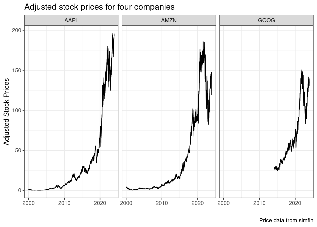
As you can see, the data is comprehensive and should suffice for many different corporate finance research topics.
5.4 Package {tidyquant}
Package {tidyquant} (Dancho and Vaughan 2023) provides functions related to financial data acquisition and analysis. It is an ambitious project that offers many solutions in the field of finance. The package includes functions for obtaining financial data from the web, manipulation of such data, and the calculation of performance measures of portfolios.
First, we will obtain price data for Apple stocks (AAPL) using function tidyquant::tq_get() .
# set stock and dates
ticker <- 'AAPL'
first_date <- '2020-01-01'
last_date <-  Sys.Date()

# get data with tq_get
df_prices <- tidyquant::tq_get(ticker,
                    get = "stock.prices",
                    from = first_date,
                    to = last_date)

dplyr::glimpse(df_prices)
R> Rows: 994
R> Columns: 8
R> $ symbol <chr> "AAPL", "AAPL", "AAPL", "AAPL", "AAPL", "…
R> $ date <date> 2020-01-02, 2020-01-03, 2020-01-06, 2020…
R> $ open <dbl> 74.0600, 74.2875, 73.4475, 74.9600, 74.29…
R> $ high <dbl> 75.1500, 75.1450, 74.9900, 75.2250, 76.11…
R> $ low <dbl> 73.7975, 74.1250, 73.1875, 74.3700, 74.29…
R> $ close <dbl> 75.0875, 74.3575, 74.9500, 74.5975, 75.79…
R> $ volume <dbl> 135480400, 146322800, 118387200, 10887200…
R> $ adjusted <dbl> 73.15265, 72.44144, 73.01869, 72.67529, 7…As we can see, except for column names, the price data has a similar format to the one we got with {yfR} (M. Perlin 2023). This is not surprising as both share the same origin, Yahoo Finance.
We can also get information about components of an index using function tidyquant::tq_index() . The available market indices are:
# print available indices
print(tidyquant::tq_index_options())
R> [1] "DOW" "DOWGLOBAL" "SP400" "SP500"
R> [5] "SP600"Let’s get information for "DOWGLOBAL".
R> Getting holdings for DOWGLOBALR> # A tibble: 179 × 8
R> symbol company identifier sedol weight sector
R> <chr> <chr> <chr> <chr> <dbl> <chr>
R> 1 QCOM QUALCOMM INC 747525103 2714… 0.00828 -
R> 2 VWS VESTAS WIND SYSTE… BN4MYF907 BN4M… 0.00810 -
R> 3 DBK DEUTSCHE BANK AG … 575035902 5750… 0.00801 -
R> 4 NKE NIKE INC CL B 654106103 2640… 0.00786 -
R> 5 BBVA BANCO BILBAO VIZC… 550190904 5501… 0.00783 -
R> 6 UCG UNICREDIT SPA BYMXPS901 BYMX… 0.00782 -
R> 7 AVGO BROADCOM INC 11135F101 BDZ7… 0.00780 -
R> 8 BA BOEING CO/THE 097023105 2108… 0.00763 -
R> 9 SPG SIMON PROPERTY GR… 828806109 2812… 0.00754 -
R> 10 SIE SIEMENS AG REG 572797900 5727… 0.00750 -
R> # ℹ 169 more rows
R> # ℹ 2 more variables: shares_held <dbl>,
R> # local_currency <chr>We only looked into a few functions from the package. {tidyquant} (Dancho and Vaughan 2023) also offers solutions for the usual financial manipulations, such as calculating returns and functions for portfolio analytics. You can find more details about this package in its website49.
5.5 Other Packages
In CRAN, you’ll find many more packages for importing financial datasets in R. In this section, we focused on packages, which are free and easy to use. Interface with commercial data sources is also possible. Several companies provide APIs for serving data to their clients. Packages such as {Rblpapi} (Armstrong, Eddelbuettel, and Laing 2022) for Bloomberg, {IBrokers} (R-IBrokers?) for Interactive Brokers can make R communicate with commercial platforms. If the company you use is not available, check the list of packages in CRAN50. It is very likely you’ll find what you need.
5.6 Accessing Data from Web Pages (webscraping)
Packages from previous section facilitates data importation over the internet. However, in many cases, the information of interest is not available through a package, but on a web page. Fortunately, we can use R to read the data and import the desired information into an R session. The main advantage is that, every time we execute the code, we get the same content available in the website.
The process of extracting information from web pages is called webscraping. Depending on the structure and technology used on the internet page, importing its content can be as trivial as a single line in R or a complex process, taking hundreds of lines of code.
5.6.1 Scraping the Components of the SP500 Index from Wikipedia
As an example of webscraping, let’s retrieve tabular information about the SP500 index from Wikipedia. In its website, Wikipedia offers a section51 about the components of the SP500 index. This information is presented in a tabular format, Figure 5.1.
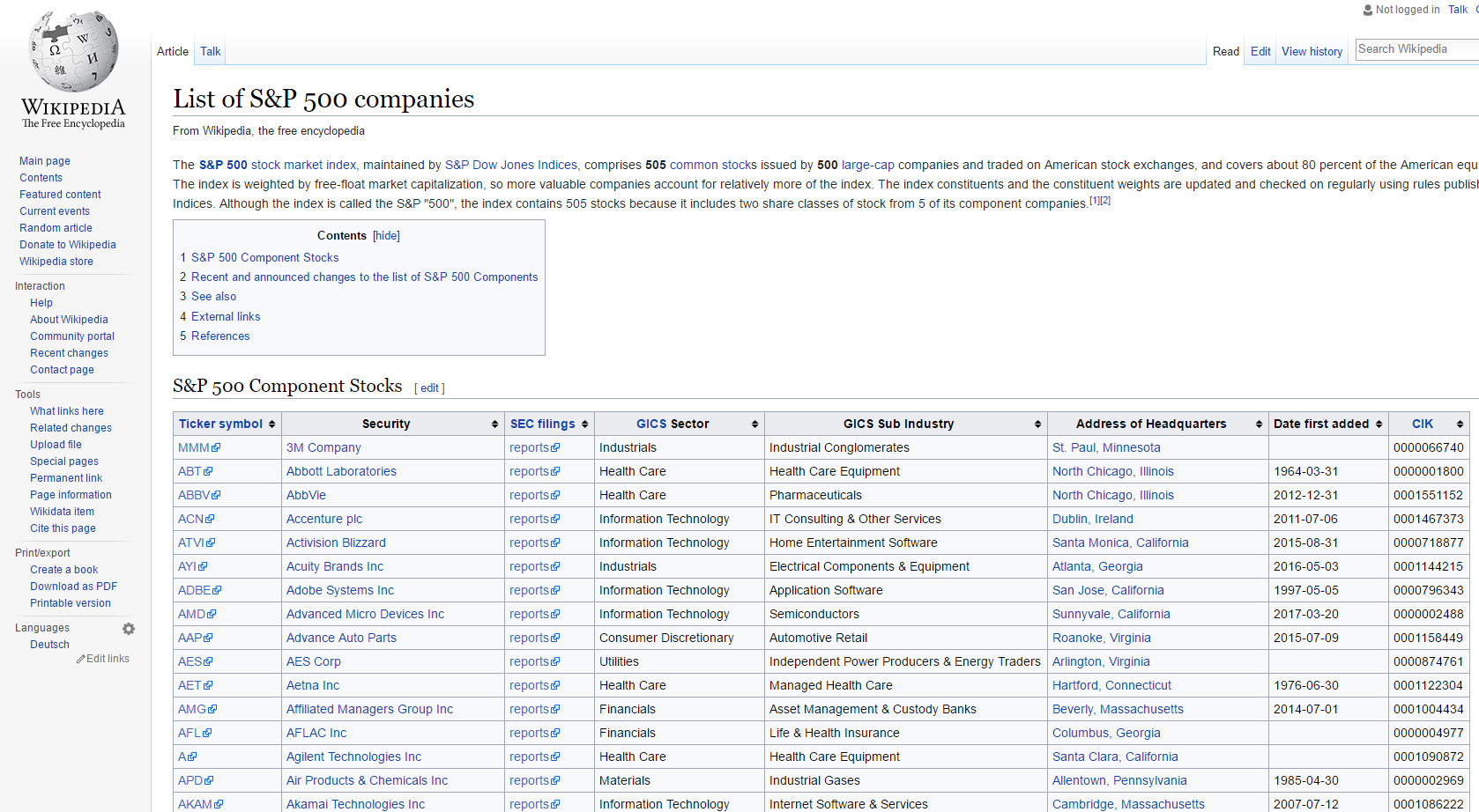
Figure 5.1: Mirror of Wikipedia page on SP500 components
The information on this web page is constantly updated, and we can use it to import information about the stocks belonging to the SP500 index. Before delving into the R code, we need to understand how a webpage works. Briefly, a webpage is nothing more than a lengthy code interpreted by your browser. A numerical value or text presented on the website can usually be found within the code. This code has a particular tree-like structure with branches and classes. Moreover, every element of a webpage has an address, called xpath. In chrome and firefox browsers, you can see the actual code of a webpage by using the mouse to right-click any part of the webpage and selecting View page source.
The first step in webscraping is finding out the location of the information you need. In Chrome, you can do that by right-clicking in the specific location of the number/text on the website and selecting inspect. This will open an extra window in the browser. Once you do that, right-click in the selection and click in copy and copy xpath. In Figure 5.2, we see a mirror of what you should be seeing in your browser.
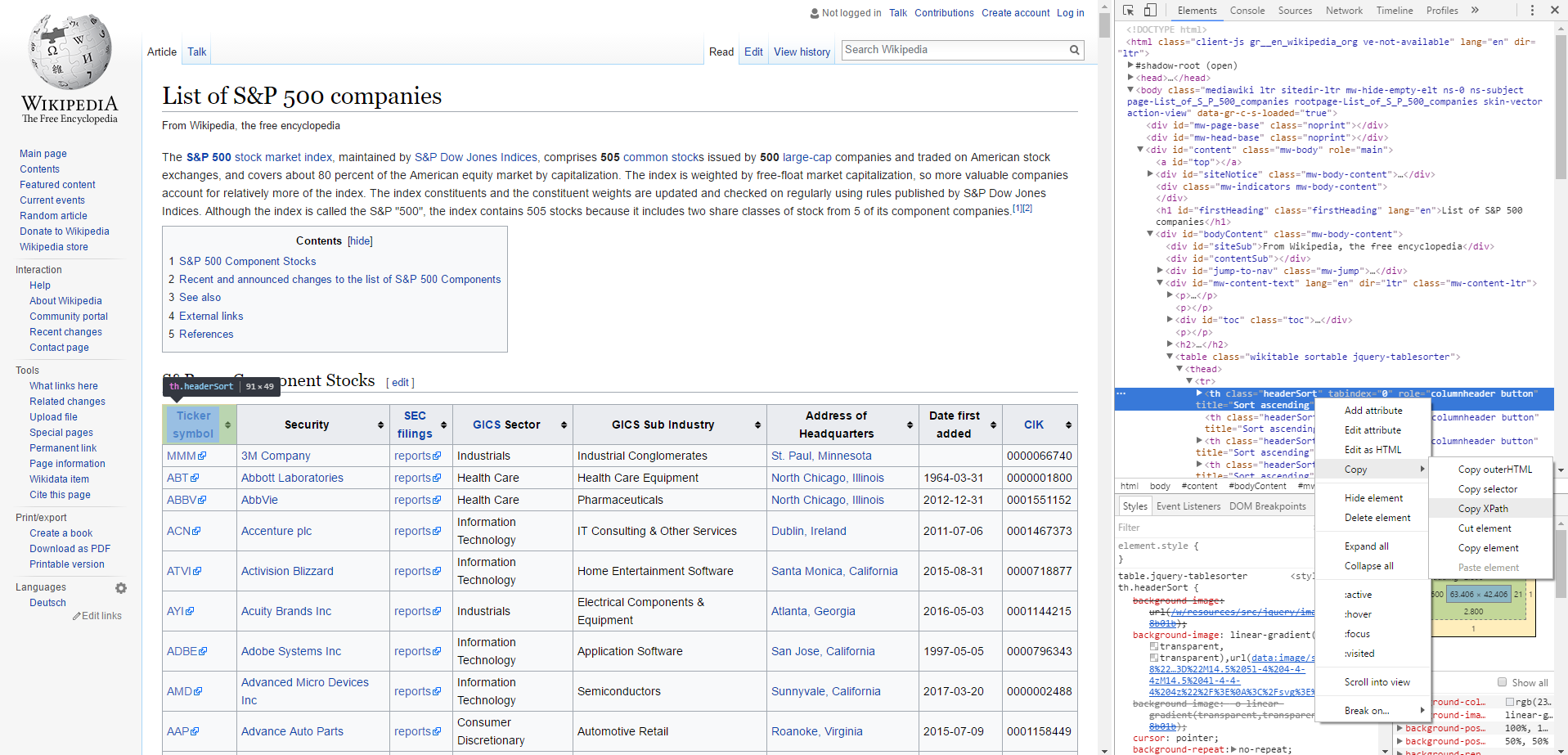
Figure 5.2: Finding xpath from website
Here, the copied xpath is:
'//*[@id="mw-content-text"]/table[1]/thead/tr/th[2]'This is the address of the header of the table. For the whole content of the table, including header, rows, and columns, we need to set an upper level of the HTML tree. This is equivalent to address //*[@id="MW-content-text"]/table[1].
Now that we have the location of what we want, let’s load package {rvest} (Wickham 2022) and use functions rvest::read_html() , rvest::html_nodes() and rvest::html_table() to import the desired table into R:
# set url and xpath
my_url <- paste0('https://en.wikipedia.org/wiki/',
                 'List_of_S%26P_500_companies')
my_xpath <- '//*[@id="mw-content-text"]/div/table[1]'

# get nodes from html
out_nodes <- rvest::html_nodes(rvest::read_html(my_url),
                        xpath = my_xpath)

# get table from nodes (each element in
# list is a table)
df_SP500_comp <- rvest::html_table(out_nodes)

# isolate it
df_SP500_comp <- df_SP500_comp[[1]]

# change column names (remove space)
names(df_SP500_comp) <- make.names(names(df_SP500_comp))

# print it
dplyr::glimpse(df_SP500_comp)
R> Rows: 503
R> Columns: 8
R> $ Symbol <chr> "MMM", "AOS", "ABT", "ABBV",…
R> $ Security <chr> "3M", "A. O. Smith", "Abbott…
R> $ GICS.Sector <chr> "Industrials", "Industrials"…
R> $ GICS.Sub.Industry <chr> "Industrial Conglomerates", …
R> $ Headquarters.Location <chr> "Saint Paul, Minnesota", "Mi…
R> $ Date.added <chr> "1957-03-04", "2017-07-26", …
R> $ CIK <int> 66740, 91142, 1800, 1551152,…
R> $ Founded <chr> "1902", "1916", "1888", "201…Object df_SP500_comp contains a mirror of the data from the Wikipedia website. The names of the columns require some work, but the raw data is intact and could be further used in a script.
Learning webscraping techniques can give you access to an immense amount of information available on the web. However, each scenario of webscraping is particular. It is not always the case you can import data directly and easily as in previous example.
Another problem is that the webscrapping code depends on the structure of the website. Any simple change in the html structure and your code will fail. You should be aware that maintaining a webscraping code can demand significant time and effort from the developer. If possible, you should always check for alternative sources of the same information.
Readers interested in learning more about this topic should study the functionalities of packages {XML} (Temple Lang 2023) and {RSelenium} (Harrison 2022)
5.7 Exercises
Q.1
Using the yfR package, download daily data of the Facebook stock (META) from Yahoo Finance for the period between 2019 and 2023. What is the lowest unadjusted closing price (column price.close) in the analyzed period?
Q.2
If you have not already done so, create a profile on the Quandl website52 and download the arabica coffee price data in the CEPEA database (Center for Advanced Studies in Applied Economics) ) between 2010-01-01 and 2020-12-31. What is the value of the most recent price?
Q.3
Use function simfinapi::sfa_get_entities() to import data about all available companies in Simfin. How many companies do you find? (see function dplyr::n_distinct()).
Q.4
With package simfinapi, download the PL (profit/loss) statement for FY (final year) data for TESLA (ticker = “TSLA”) for year 2022. What is the latest Profit/Loss of the company for that particular year?
Q.5
Using function tidyquant::tq_index, download the current composition of index SP400. What is the company with the highest percentage in the composition of the index?
Be aware that the answer is time-dependent and the reported result might be different from what you actually got in your R session.
Q.6
Using again the yfR package, download financial data between 2019-01-01 and 2020-01-01 for the following tickers:
- AAPL: Apple Inc
- BAC: Bank of America Corporation
- GE: General Electric Company
- TSLA: Tesla, Inc.
- SNAP: Snap Inc.
Using the adjusted closing price column, what company provided higher return to the stock holder during the analyzed period?
Tip: this is an advanced exercise that will require some coding. To solve it, check out function split to split the dataframe of price data and lapply to map a function to each dataframe.